Modeling the circulation and dispersion in
Santos coastal region (SP, Brazil):
applications to impacted and preserved areas
Joseph Harari & Ricardo de Camargo & Carlos Augusto de Sampaio França &
Mauro Quandt Monteiro
joharari@usp.br , ricamarg@model.iag.usp.br ,
cafranca@usp.br , brum@io.usp.br
Instituto Oceanográfico da USP, São Paulo, SP, Brasil
Tel. +55-11-3091.6576, Fax +55-11-3091.6610
I. INTRODUCTION
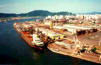
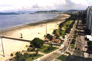
The coastal region of Santos (Sao Paulo State, Brazil) is an important complex with large population, significant economic developments, beautiful beaches for tourism and, most important, the largest port of South America. Its geomorphology and industrial activities cause serious problems of pollution, both in the air and sea environments. The map of the area is shown on Figure 1 and views of the port and beaches are on Figure 2.
One of the important environmental aspects is related to pollution in the ocean outfall area; this outfall is 4000 m long, placed at 11.0 m depth, with a diffuser length of 200 m, 40 ports spaced at 5 m intervals, having an initial dilution < 30; its position is shown on Figure 3.
On the other hand, in this coastal area is located the "Parque Estadual Marinho da Laje de Santos" (The State Marine Preservation Park of Santos Flagstone), with an area of 5000 hectares (50 Km2), about 20 miles (37 Km) South of Santos (Figure 3); this area is a shelter for several species of birds and fishes and has been protected from any human intervention and occupation (see views on Figure 4).
For the coastal area of Santos as a whole, many scientific and technical projects were executed in the last years, aiming to preserve, as far as possible, its environmental resources and the quality of life of inhabitants and tourists. These projects were mainly related to dredging operations in the channel of the Port (in order to assure the security of large vessels), monitoring the outfall operation (and water quality surveys) and the evolution of the sand beaches (to prevent coastal erosion).
One of these projects (carried out in the period 2002 / 2003) was "A preliminary biological and oceanographic survey in the area of The State Marine Preservation Park of Santos Flagstone", with the objective of developing scientific studies in the area and, in the long term, to contribute for its preservation (Machado, Harari & Oliveira, 2003; Harari, Gonzalez & Sampaio, 2003).
As components of these projects, several numerical models have been used to represent the hydrodynamics of this coastal area, with many applications, such as support to navigation security, water quality monitoring and sediment transport estimates. Some results of numerical simulations are here presented, with emphasis on the dispersion in the outfall area and the circulation components in the protected region of "Laje de Santos".
Fig. 1 – Geographic map of the coastal area of Santos (SP, Brazil).
|
|
Fig. 2 – Views of the port and beaches of Santos.
Fig. 3 – Bathymetry of the coastal area of Santos and location of the ocean outfall and the "Laje de Santos" (flagstone of Santos).
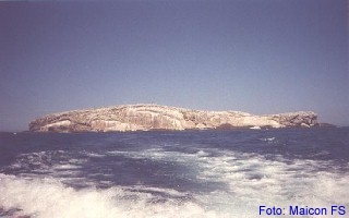
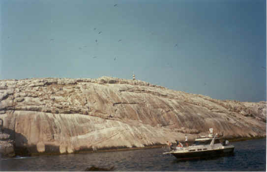
Fig. 4 – Views of "Laje de Santos" (Santos flagstone).
II. METHODOLOGY
The numerical simulations of the coastal circulation were performed with a model based on the Princeton Ocean Model - POM (Blumberg & Mellor, 1987), considering several forcing combinations (of tides, winds and density effects); this model was used on researches concerning the coastal area of Santos, by Harari & Camargo (1997, 1998, 2003), Harari, Camargo & Cacciari (2000) and Harari, Camargo & Miranda (2002).
POM is a three-dimensional non-linear model with the complete hydrodynamic equations (for sea surface level, currents, temperature, salinity and density), which solution is obtained on sigma vertical coordinates (that follow the bottom relief), considering modes splitting and a second order turbulent closure (Mellor, 1998). The numerical solution adopts a centered explicit scheme, for the time and horizontal space domains, and an implicit scheme, for the vertical domain (Kowalik & Murty, 1993).
The model runs considered tidal effects (spring and neap tide periods), meteorological influences (predominant conditions and winds generated by intense cold fronts) and sea water density effects (including river discharges); several combinations of tides, winds and density were considered, for typical (mean) and extreme events.
For the boundary conditions of the circulation model, tides are specified by a coarser numerical model of the shelf (Harari & Camargo, 1994); winds at the surface are given by the atmospheric numerical model of the National Climate and Environmental Prediction – NCEP, USA, with resolution of 6 hours in time and between 200 and 250 Km in space, with hourly interpolations for each point of the coastal oceanic grids; density values are prescribed as monthly climatological means (Levitus & Boyer, 1994). Mean sea level oscillations at the boundaries are based on coastal measurements in the Port of Santos (Harari & Camargo, 1995) and operational predictions in the Southwest Atlantic regularly available on http://www.surge.iag.usp.br (Camargo et al, 2000).
The dispersion model (Harari, Camargo & Gordon, 2000; Harari & Gordon, 2001) solves the advection – diffusion – decay equation of an initial concentration (with continuous sources); this model makes use of the same grid and numerical schemes of the hydrodynamic one. This equation represents the dispersion of a substance (or pollutant) in vertical equilibrium with the surrounding environment, thus there is no forced jet or buoyancy; the model is therefore concerned with the "far field", and not the "near field", which consists of the initial times of ejection of substances into the sea (Proctor et al, 1994; Ahsan et al, 1994). Any decay rate of a contaminant may be specified in the model (with typical values of T90 given as 8, 6 and 2 hours)
In this presentation, the first grid is centered on the outfall area and includes the Port of Santos and internal shallow region (see Figure 3 for details). The mesh has maximum depth of 15 m, axis inclination of 62° relative to the EW direction, being formed by 150 x 164 points, with variable horizontal spacing (minimum value of 96 m) and 11 vertical sigma levels, placed at the following fractions of the total depth: 0, 0.03125, 0.0625, 0.125, 0.25, 0.5, 0.75, 0.875, 0.9375, 0.96875 e 1.0. The external mode has a time step of 2 s and the internal ones of 30 s.
The second grid covers the "Laje de Santos" area, with 200 x 200 points, constant spacings of 72 m in the EW direction and 93 m in the NS, and the same 11 sigma levels of the former grid. Its bathymetry is shown on Figure 5, with maximum depth of 48.8 m; time steps of 30 s and 1 s were adopted, for the internal and external modes of oscillation, respectively.
III. RESULTS
As an example of the results obtained by the circulation and dispersion models, the evolution of currents and plume are presented, for a numerical experiment relative to the period of 15 to 25 January 2001, when tides change from neap to spring regimes, with additional significant variations of mean sea level, as can be observed on Figure 6.
A theoretical pollutant is ejected on 00 GMT 17 January, with a vertical profile having maximum at 8.25 m (50% of the discharge), intermediate values at 5.5 m and 9.625 m (20% each) and minimum values at 2.75 m e 10.31 m (5% each); afterwards, a constant in time ejection is considered, each hour having 36% of the initial value, with the same vertical distribution.
Fig. 5 – Bathymetry of the grid covering the "Laje de Santos" area (m).
Fig. 6 – Sea level elevation computed by the model in the Port of Santos, on grid point (column, line = 60, 105) with coordinates 46.34° W 23.92° S (see Figures 7a, b).
Fig. 7a – Currents (m/s) and surface concentrations (see color bar) after 6 hours of pollutant release.
Fig. 7b – Currents (m/s) and surface concentrations (see color bar) after 12 hours of pollutant release.
Figures 7a, b display the time variation of currents and percentile distributions computed by the model, at the surface, after 6 and 12 hours of the ejection beginning (considering no concentration decay). The results show the pollutant transport and spreading, in a period of strong ebbing currents, due to tides and meteorological effects, driving the pollutant that reached the surface to the open sea. Note that the concentrations that reach the surface present minimum values and surely would be smaller in case of concentrations decay (with T90 values of 6 or 2 hours, for example).
Figure 8 shows surface currents computed by the grid covering the "Laje de Santos" area, in a period of spring tides, considering instantaneous maximum flooding tides (02 GMT de 08 de Janeiro de 1997); this figure display every 5th horizontal vector generated by model runs, considering forcings of tides; winds; tides and winds; and finally tides, winds and density effects. The maps show the influence of bathymetry and the emerged part of the flagstone in the currents distributions; besides, there are strong interactions of meteorological and density effects with the tidal circulation. At the specific time of the figure, the tidal currents are basically to Northwest, wind currents flow to the West, but the density currents produce a general pattern to the Southwest.
IV. CONCLUSIONS
Numerical modeling is an important tool for environmental studies and preservation. The hydrodynamic characteristics affect the concentrations of pollutants or properties, with displacements that follow the tidal ebbing and flooding, as well as the wind and density currents. It also may help to delimit areas that may suffer impacts due to environmental accidents.
Efforts have been made to use the hydodynamical and dispersion models in standard and operational patterns, with systematic simulations of the dispersion, using read data of pollutants discharges regularly made available by the governmental agency (Cetesb, 2001, 2004), which will allow several applications in engineering and environmental sciences, especially on the water quality control.
REFERENCES
AHSAN, A. K. M. Q.; BRUNO, M. S.; OEY, L-Y. and HIRES, R. I. 1994. Wind-driven dispersion in New Jersey coastal waters. Journal of Hydraulic Engineering, 120(11), 1264-1273.
BLUMBERG, A.F. & MELLOR, G.L. 1987. A description of a three-dimensional coastal ocean circulation model. In: Three-Dimensional Coastal Ocean Models, Vol. 4, p. 1 – 16, American Geophysical Union, Washington D.C., USA, 208p.
CAMARGO, R. & HARARI, J. & DIAS, P. L. S. & CARUZZO, A. & ZACHARIAS, D. C. - 2000 - "Implementação de sistema de previsão de marés meteorológicas no Atlântico Sudoeste" – (digital format) XI Congresso Brasileiro de Meteorologia, Rio de Janeiro (RJ), October 2000, p. 2646 - 2654.
CETESB 2001 - Sistema Estuarino de Santos e São Vicente, Relatório Técnico DAH, 178 p + 42 mapas.
CETESB 2004 – Relatório de qualidade das águas litorâneas do Estado de São Paulo: balneabilidade das praias 2003 / CETESB – São Paulo. CD rom, 183 p.
HARARI, J. & CAMARGO, R. - 1994 - "Simulação da propagação das nove principais componentes de maré na plataforma sudeste brasileira através de modelo numérico hidrodinâmico" - Boletim do Instituto Oceanográfico da USP, n° 42 (1), p. 35 - 54.
HARARI, J. & CAMARGO, R. - 1995 - "Tides and mean sea level variabilities in Santos (SP), 1944 to 1989" - Relatório Interno do Instituto Oceanográfico da USP, n° 36, 15 p.
HARARI, J. & CAMARGO, R. - 1997 - "Simulações da circulação de maré na região costeira de Santos (SP) com modelo numérico hidrodinâmico" - Pesquisa Naval - Suplemento Especial da Revista Marítima Brasileira, n° 10, p. 173 - 188.
HARARI, J. & CAMARGO, R. - 1998 - "Modelagem numérica da região costeira de Santos (SP): circulação de maré" - Revista Brasileira de Oceanografia, vol. 46 (2), p. 135 - 156.
HARARI, J. & CAMARGO, R. - 2003 - "Numerical simulation of the tidal propagation in the coastal region of Santos (Brazil, 24° S 46°W)" - Continental Shelf Research, vol. 23 (2003), p. 1597 – 1613.
HARARI, J. & CAMARGO, R. & CACCIARI, P. L. – 2000 - "Resultados da modelagem numérica hidrodinâmica em simulações tridimensionais das correntes de maré na Baixada Santista" - Revista Brasileira de Recursos Hídricos, vol. 5, n° 2, p. 71 – 87.
HARARI, J. & CAMARGO, R. & GORDON, M. - 2000 - "Numerical simulations of the hydrodynamics and the dispersion of substances in the coastal area of Santos (SP, Brazil)" – digital format - ICECE 2000 - International Conference on Engineering and Computer Education, São Paulo (SP), Brasil, September 2000, 4p.
HARARI, J. & CAMARGO, R. & MIRANDA, L. B. - 2002 - "Modelagem numérica hidrodinâmica tridimensional da região costeira e estuarina de São Vicente e Santos (SP)" - Pesquisa Naval - Suplemento Especial da Revista Marítima Brasileira, n° 15, p. 79 - 97.
HARARI, J. & GONZALEZ, F. S. & SAMPAIO, A. F. P. – 2003 – "O Projeto ‘Vida na Laje de Santos’ – Subprojeto Oceanografia Física / Hidrodinâmica" - Resume (T205) – digital format - III Congresso Brasileiro de Pesquisas Ambientais e Saúde – III CBPAS, Santos (SP, Brasil), July 2003, p. 117 a 121.
HARARI, J. & GORDON, M. - 2001 - "Simulações numéricas da dispersão de substâncias no Porto e Baía de Santos, sob a ação de marés e ventos" - Revista Brasileira de Recursos Hídricos, vol. 6, n° 4, p. 115 – 131.
KOWALIK, Z. & MURTY, T. S. - 1993 - "Numerical modeling of ocean dynamics" - World Scientific - Advanced Series on Ocean Engineering, vol. 5, 481 p.
LEVITUS, S & BOYER, T. P. – 1994 – "World Ocean Atlas 1994" – Technical Report vol. 4, National Oceanographic Data Center, Ocean Climate Laboratory, 117 p.
MACHADO, M. B. & HARARI, J. & OLIVEIRA, M. R. – 2003 – "Projeto Vida na Laje: Levantamento preliminar biológico e oceanográfico da área do Parque Estadual Marinho da Laje de Santos" - Resume (T193) – digital format - III Congresso Brasileiro de Pesquisas Ambientais e Saúde – III CBPAS, Santos (SP, Brasil), July 2003, 4 p.
Mellor, G. L., 1998. A three-dimensional, primitive equation, numerical ocean model – User’ s Guide. Princeton University, Internal Report, 41 p.
PROCTOR, R. & FLATHER, R. A. & ELLIOT, A. J. – 1994 – "Modelling tides and surface drift in the Arabian Gulf - Applications to the gulf oil spill" - Continental Shelf Research, Vol. 14, n° 5, pp 531-545.
Fig. 8 – Sea surface level (meters, see color bar) and instantaneous surface currents (m/s), in spring tide period, computed by the model with the following forcings: tides (top left), winds (top right), tides and winds (bottom left) and tides, winds and density (bottom right) – plot of every 5th vector computed by the model.